Features

Apart from getting the timings, we can further process the underlying data to study various aspects of the benchmarking.

Speedups & scaled-timings

Benchmarking results could be stored as two more datatypes with BenchmarkObj, namely speedups and scaled_timings (timings numbers simply scaled by one reference function). So, these alongwith the entry datatype of timings form the essential three datatypes of this package. All asssociated class methods and utility functions revolve around them.

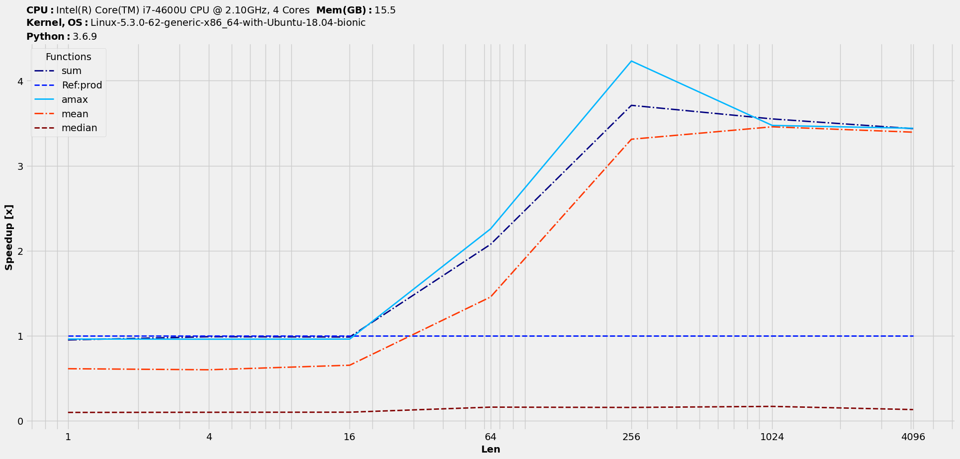
Let’s study the speedups of all w.r.t prod alongwith ranking :

>>> s = t.speedups(ref=1) # prod's location index in t is 1
>>> s.plot(logy=False, logx=True, save='speedups_by_prod.png')

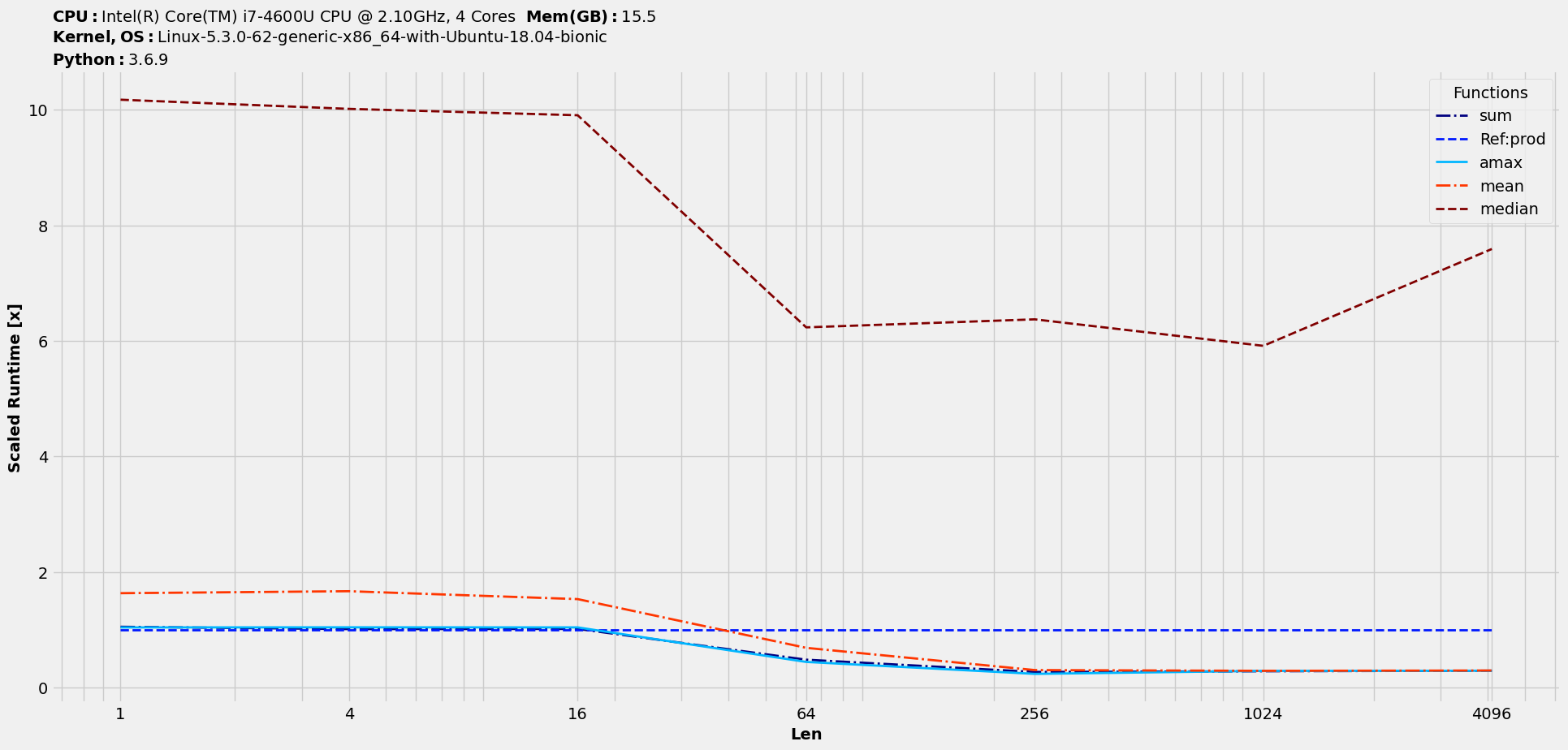
Finally, the scaled-timings :

>>> st = t.scaled_timings(ref=1) # prod's location index in t is 1
>>> st.plot(logy=False, logx=True, save='scaledtimings_by_prod.png')

The input argument to methods speedups and scaled_timings i.e. ref accepts three types of arguments for indexing - int as the location index, str as the function name string and function itself that was input into funcs.

Let’s explore the other available tools with this package. As mentioned earlier, all of these are applicable to all the three datatypes with BenchmarkObj. We will re-use the numbers obtained with the Minimal workflow discussed earlier.

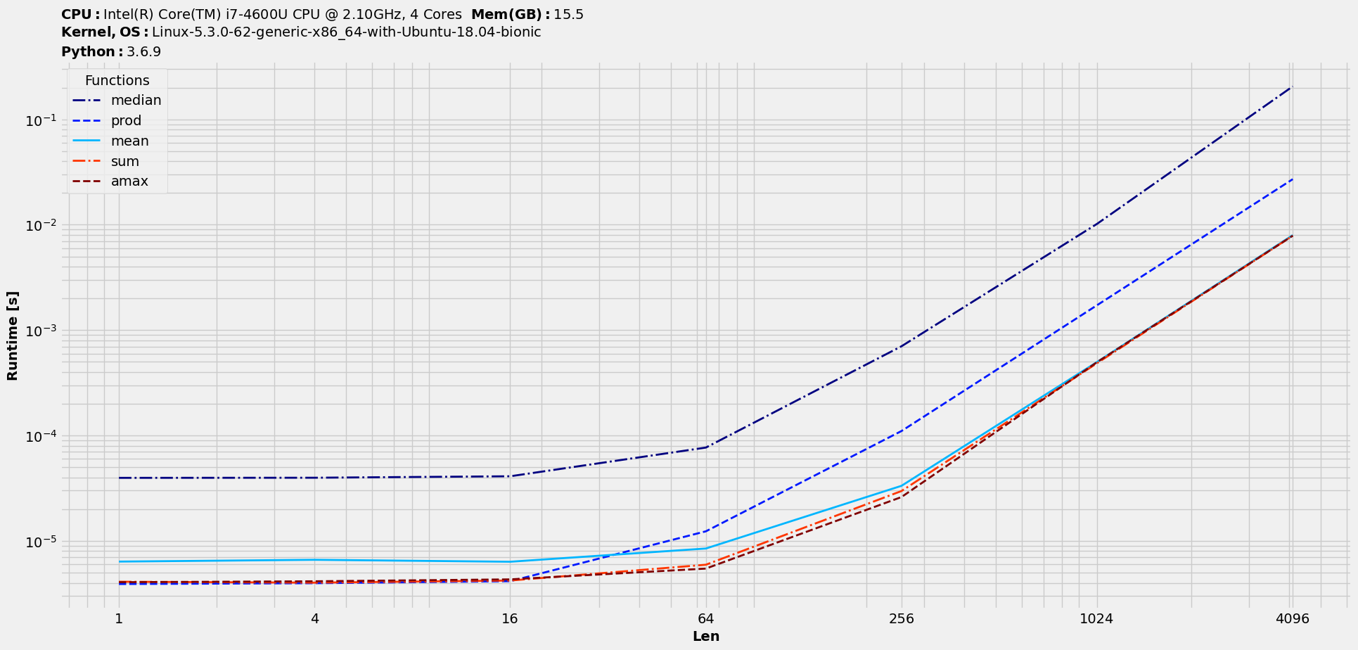
Rank & reset_columns

The order of the plot legend by default would be same as the order in funcs argument. With many competing solutions in funcs, for an easy correlation between them and the plot lines, we might want to sort the legend based on their performance and hence comes the idea of ranking. There are various criteria on which performance could be ranked. Let’s explore the usage with the default one :

>>> t.rank()
>>> t.plot(logy=True, logx=True, save='timings_ranked.png')

Note that ranking would have changed the columns order. To revert to the original order, use :

>>> t.reset_columns()

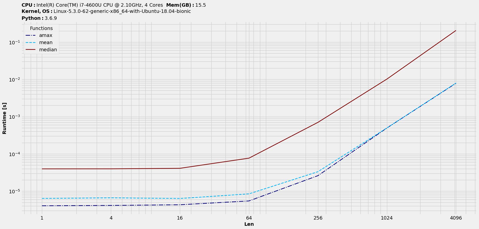
Drop

Let’s say we might want to focus on few functions and hence drop the others or even drop some input datasets. This method does the job, as we can drop by the column and index values. Note that this works in-place. So, if we want to drop median and prod, it would be :

>>> t.drop(['sum', 'prod'], axis=1)
>>> t.plot(logy=True, logx=True, save='timings_dropfuncs.png')

To drop certain datasets (starting with original t) :

>>> t.drop([1,16], axis=0)
>>> t.plot(logy=True, logx=True, save='timings_dropdata.png')

Copy

As the name suggests, we can make a copy of the benchmarking object with it. It should be useful when we are trying out stuffs and need a backup of benchmarking results.

Expose to pandas-world

Earlier we saw how we can go back and forth between benchit.BenchmarkObj and pandas.DataFrame. We also studied how that could be used to extend plot functionality. In this section, let’s study how we can extend it to manipulate benchmarking results. We will continue with the hands-on method of explanation.

General syntax

For a given benchmarking object t, the general syntax on working with the underlying dataframe would be something like this :

>>> df = t.to_dataframe()
>>> df_new = # some operation on df to result in a new dataframe, df_new
>>> benchit.bench(df_new, dtype=t.dtype)

Examples

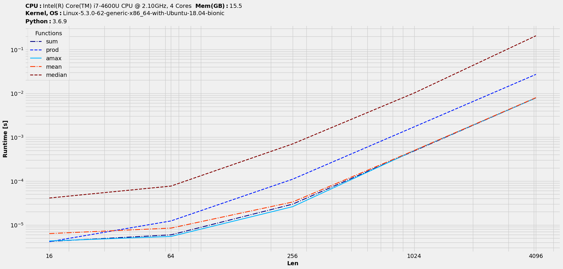
We will take over from Minimal workflow with the timings plot and look at few cases. For reference, the timings plot looked something like this :

Crop

As an example, just to emphasize on the ease to do this business, a typical way of dropping the first two datasets would be :

>>> benchit.bench(t.to_dataframe().iloc[2:],dtype=t.dtype)

Default dtype argument for benchit.bench is set for timings. So, it becomes simpler with :

>>> benchit.bench(t.to_dataframe().iloc[2:]).plot(logx=True, save='timings_cropdata.png')

Combine

Back to the same Minimal benchmarking workflow, let’s say we want to see the combined timings for two functions and how would it fare against other individual functions. Dataframe format makes it easy :

# Create a new column with combined data
>>> df['sum+amax'] = df['sum'] + df['amax']

# Create a new function-column with combined data and plot
>>> benchit.bench(df).plot(logx=True, save='timings_comb.png')

At least one interesting observation could be made there. If we compare combined one of sum & max against prod, the former wins on lower timings only with larger datasets.

Earlier listed Drop is based on this strategy of working with the inherent dataframe data. There are endless possibilities and scenarios where having a dataframe data could be useful and necessary!