Real-world examples

We will take few realistic scenarios and also study how arguments could be setup differently.

Multiple arg

Adding arrays

We will study a multiple argument case. This was inspired by a Stack Overflow question on adding two arrays. We will study the case of functions that accept two arguments. The two functions in consideration are :

def new_array(a1, a2):
    a1 = a1 + a2

def inplace(a1, a2):
    a1 += a2

These accept NumPy array data and thus would perform those summations and write-back in a vectorized way. The first one does summation stores in temporary buffers and then pushes back the result to a new memory space, while the second method writes back the addition result to first array’s memory space. We are investigating, which one’s better and by how much. Let’s put them to the test using our tools!

Now, as mentioned earlier, for multiple argument cases, we need to feed in each of those input datasets as a tuple each. We could setup the inputs as a list. But, let’s setup in a dictionary, so that datasets are assigned labels with its keys. Let’s get the timings and hence plot them :

>>> R = np.random.rand
>>> inputs = {(i,i):(R(i,i),R(i,i)) for i in 2**np.arange(3,13)}
>>> t = benchit.timings([new_array,inplace], inputs, multivar=True, input_name='Array-shape')
>>> t.plot(logy=True, logx=False, save='multivar_addarrays_timings.png')

Looking at the plot, we can conclude that the write-back one is better for larger arrays, which makes sense given its memory efficiency.

Euclidean distance

Single variable

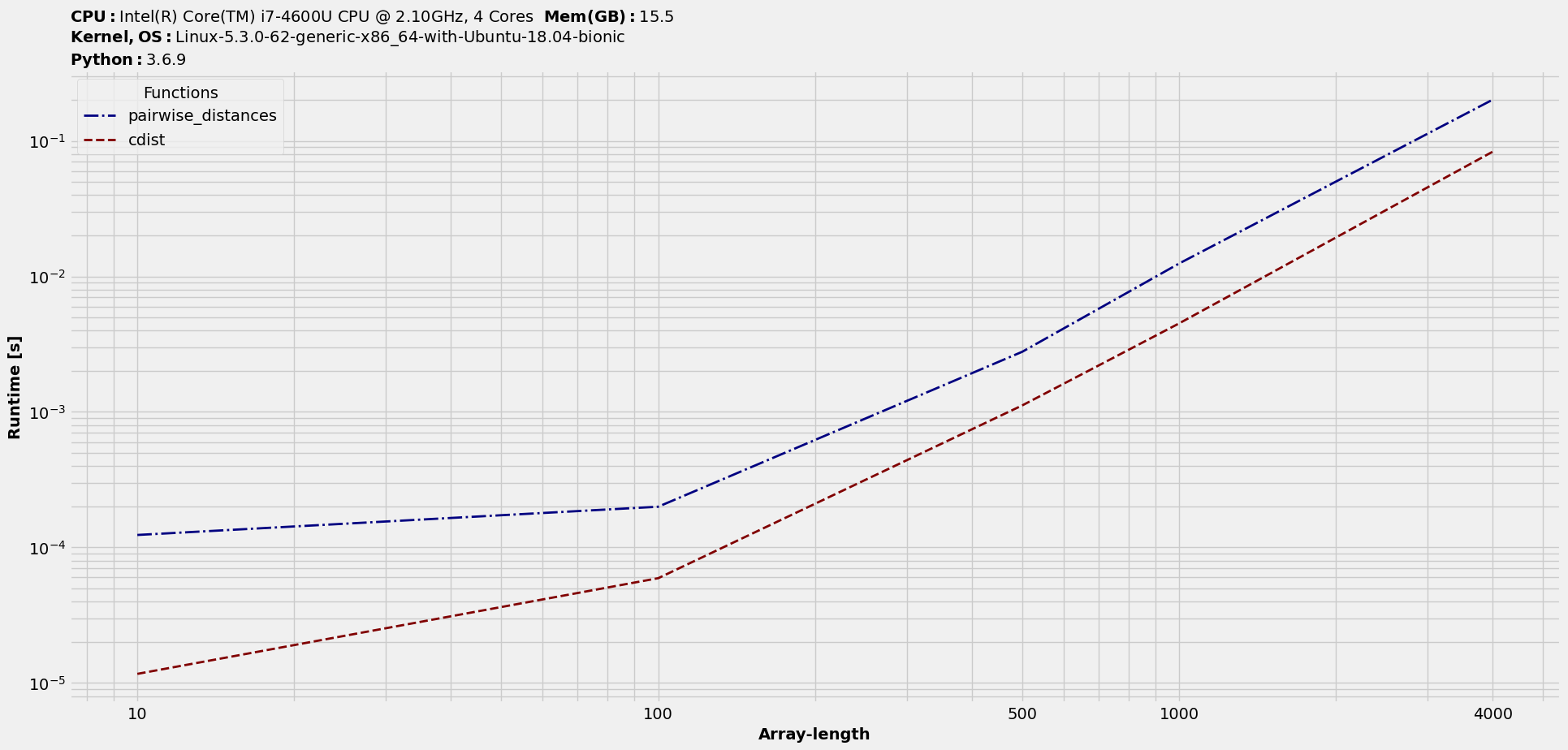
We will study another multiple argument case. The setup involves euclidean distances between two 2D arrays. We will feed in arrays with varying number of rows and 3 columns to represent data in 3D Cartesian coordinate system and benchmark two commonly used functions in Python.

# Setup input functions
>>> from sklearn.metrics.pairwise import pairwise_distances
>>> from scipy.spatial.distance import cdist
>>> fns = [pairwise_distances, cdist]

# Setup input datasets
>>> import numpy as np
>>> in_ = {n:[np.random.rand(n,3), np.random.rand(n,3)] for n in [10,100,500,1000,4000]}

# Get benchmarking object (dataframe-like) and plot results
>>> t = benchit.timings(fns, in_, multivar=True, input_name='Array-length')
>>> t.plot(save='multivar_euclidean_timings.png')

Multi-variable Groupings

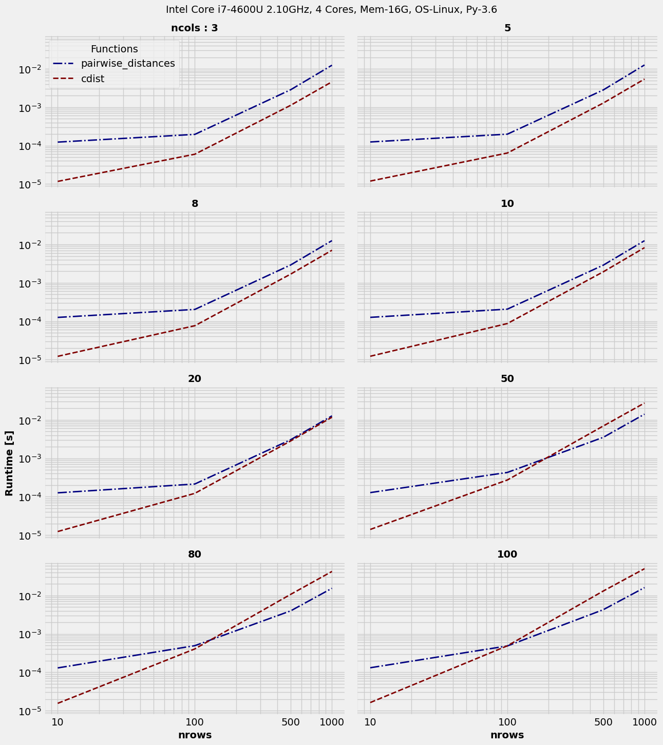
We will simply extend previous test-case to cover for the second argument to the distance functions, i.e. with varying number of columns. We will re-use most of that earlier setup.

Also, we will explore subplot specific arguments available with plot. These are marked with prefix as : sp_, short for subplot_.

>>> R = np.random.rand
>>> nrows_list = [10, 100, 500, 1000]  # list of number of rows
>>> ncols_list = [3, 5, 8, 10, 20, 50, 80, 100]  # list of number of cols
>>> in_ = {(nr,nc):[R(nr,nc), R(nr,nc)] for nr in nrows_list for nc in ncols_list}
>>> t = benchit.timings(fns, in_, multivar=True, input_name=['nrows', 'ncols'])

Now, let’s do the groupings to study the behaviour w.r.t. to each argument.

Grouping based on argID = 0 :

>>> t.plot(logx=True, sp_ncols=2, sp_argID=0, sp_sharey='g', save='multigrp_id0_euclidean_timings.png')

Grouping based on argID = 1 :

>>> t.plot(logx=True, sp_ncols=2, sp_argID=1, sp_sharey='g', save='multigrp_id1_euclidean_timings.png')

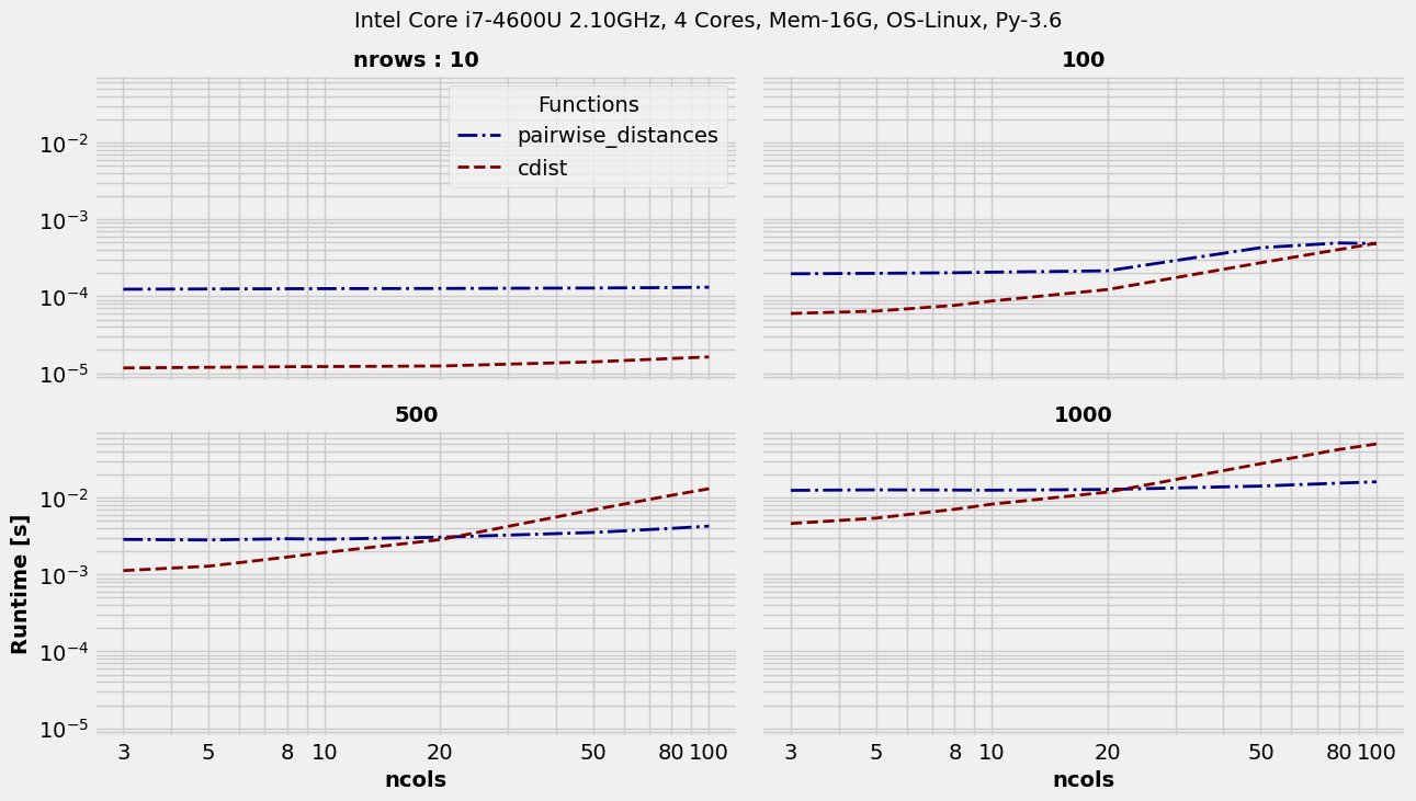
Some interesting obseravtions could be made there. The implementations are obviously different. This is resulting in pairwise_distances winning as we move to higher number of columns. Though, on smaller datasets or with smaller number of rows, cdist is clearly ahead.

Single arg

Forward-fill on mask

Single-variable Groupings

Let’s manufacture a simple forward-filling scheme based on indices of True values in a boolean-array, whereas False should keep previous values. Also, the values would be kept as 0s until the first True.

To give it a better understanding, two examples should clarify with a solution based on np.maximum.accumulate :

>>> b
array([ True, False,  True,  True, False, False, False,  True, False, False])
>>> np.maximum.accumulate(np.where(b,np.arange(len(b)), 0))
array([0, 0, 2, 3, 3, 3, 3, 7, 7, 7])

>>> b
array([False, False, False,  True, False, False, False,  True, False, False])
>>> np.maximum.accumulate(np.where(b,np.arange(len(b)), 0))
array([0, 0, 0, 3, 3, 3, 3, 7, 7, 7])

We could also solve it with np.repeat based on the counts between consecutive True ones. Let’s benchmark these two methods :

# Functions
def repeat(b):
    idx = np.flatnonzero(np.r_[b,True])
    return np.repeat(idx[:-1], np.diff(idx))

def maxaccum(b):
    return np.maximum.accumulate(np.where(b,np.arange(len(b)), 0))

in_ = {(n,sf): np.random.rand(n)<(100-sf)/100. for n in [100,1000,10000,100000,1000000] for sf in [20, 40, 60, 80, 90, 95]}
t = benchit.timings([repeat, maxaccum], in_, input_name=['Array-length','Sparseness %'])
t.plot(logx=True, sp_ncols=2, save='singlegrp_id0_ffillmask_timings.png')

As always, some interesting inferences could be derived there. Seems np.maximum.accumulate is winning on most occasions, whereas repeat based one is doing better on highly sparse big datasets.

No argument

Random sampling

Finally, there might be cases when input functions have external no argument required. To create one such scenario, let’s consider a setup where we compare numpy.random.choice against random.sample to get samples without replacement. We will consider an input data of 1000,000 elements and use those functions to extract 1000 samples. We will test out random.sample with two kinds of data - array and list, while feeding only array data to numpy.random.choice. Thus, in total we have three solutions, as listed in the full benchmarking shown below :

# Global inputs
import numpy as np
ar = np.arange(1000000)
l = ar.tolist()
sample_num = 1000

# Setup input functions with no argument
# NumPy random choice on array data
def np_noreplace():
    return np.random.choice(ar, sample_num, replace=False)

from random import sample

# Random sample on list data
def randsample_on_list():
    return sample(l, sample_num)

# Random sample on array data
def randsample_on_array():
    return sample(ar.tolist(), sample_num)

# Benchmark
t = benchit.timings(funcs=[np_noreplace, randsample_on_list, randsample_on_array])
>>> t
Functions  np_noreplace  randsample_on_list  randsample_on_array
Case
NoArg           0.02528            0.000653             0.033294

One interesting observation there - With array data numpy.random.choice is slightly better than random.sample. But, if we allow the flexibility of choosing between list and array data, random.sample turns the table in a big way. That’s the whole point with benchmarking, which is to get insights into how different modules compare on the same functionality and how different data formats affect those runtime numbers. This in turn, should help the end-user decide on choosing methods depending on the available setup.